Data Structure – Graphs
Graph G is a pair (V, E), where V is a finite set of vertices and E is a finite set of edges. We will often denote n = |V|, e = |E|.
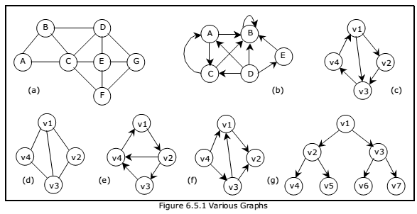
A graph is generally displayed as figure 6.5.1, in which the vertices are represented by circles and the edges by lines.
An edge with an orientation (i.e., arrow head) is a directed edge, while an edge with no orientation is our undirected edge.
If all the edges in a graph are undirected, then the graph is an undirected graph. The graph in figure 6.5.1(a) is an undirected graph. If all the edges are directed; then the graph is a directed graph. The graph of figure 6.5.1(b) is a directed graph. A directed graph is also called as digraph. A graph G is connected if and only if there is a simple path between any two nodes in G
A graph G is said to be complete if every node a in G is adjacent to every other node v in G. A complete graph with n nodes will have n(n-1)/2 edges. For example, Figure 6.5.1.(a) and figure 6.5.1.(d) are complete graphs.
A directed graph G is said to be connected, or strongly connected, if for each pair (u, v) for nodes in G there is a path from u to v and also a path from v to u. On the other hand, G is said to be unilaterally connected if for any pair (u, v) of nodes in G there is a path from u to v or a path from v to u. For example, the digraph shown in figure 6.5.1 (e) is strongly connected.
We can assign weight function to the edges: Wg(e) is a weight of edge e ∈ E. The graph which has such function assigned is called weighted graph.
The number of incoming edges to a vertex v is called in–degree of the vertex (denote indeg(v)). The number of outgoing edges from a vertex is called out-degree (denote outdeg(v)). For example, let us consider the digraph shown in figure 6.5.1(f),
indegree(v1) = 2
outdegree(v1) = 1
indegree(v2) = 2
outdegree(v2) = 0
A path is a sequence of vertices (v1, v2, . . . . . , vk), where for all i, (vi, vi+1) ε E. A path is simple if all vertices in the path are distinct. If there is a path containing one or more edges which starts from a vertex Vi and terminates into the same vertex then the path is known as a cycle. For example, there is a cycle in figure 6.5.1(a), figure 6.5.1(c) and figure 6.5.1(d).
If a graph (digraph) does not have any cycle then it is called acyclic graph. For example, the graphs of figure 6.5.1 (f) and figure 6.5.1 (g) are acyclic graphs.
A graph G’ = (V’ , E’ ) is a sub-graph of graph G = (V, E) iff V’ ⊆ V and E’ ⊆ E.
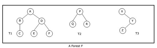
A Forest is a set of disjoint trees. If we remove the root node of a given tree then it becomes forest. The following figure shows a forest F that consists of three trees T1, T2 and T3.
A graph that has either self loop or parallel edges or both is called multi-graph.
Tree is a connected acyclic graph (there aren’t any sequences of edges that go around in a loop). A spanning tree of a graph G = (V, E) is a tree that contains all vertices of V and is a subgraph of G. A single graph can have multiple spanning trees.
Let T be a spanning tree of a graph G. Then
- Any two vertices in T are connected by a unique simple path.
- If any edge is removed from T, then T becomes disconnected.
- If we add any edge into T, then the new graph will contain a cycle.
- Number of edges in T is n-1.
Representation of Graphs:
There are two ways of representing digraphs. They are:
- Adjacency matrix.
- Adjacency List.
- Incidence matrix.
Adjacency matrix:
In this representation, the adjacency matrix of a graph G is a two dimensional n x n
matrix,
The matrix is symmetric in case of undirected graph, while it may be asymmetric if the
graph is directed. This matrix is also called as Boolean matrix or bit matrix.
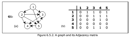
Figure 6.5.2(b) shows the adjacency matrix representation of the graph G1 shown in
figure 6.5.2(a). The adjacency matrix is also useful to store multigraph as well as
weighted graph. In case of multigraph representation, instead of entry 0 or 1, the entry
will be between number of edges between two vertices.
In case of weighted graph, the entries are weights of the edges between the vertices.
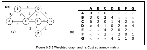
The adjacency matrix for a weighted graph is called as cost adjacency matrix. Figure
6.5.3(b) shows the cost adjacency matrix representation of the graph G2 shown in
figure 6.5.3(a).
Adjacency List:
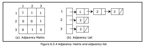
In this representation, the n rows of the adjacency matrix are represented as n linked
lists. An array Adj[1, 2, . . . . . n] of pointers where for 1 < v < n, Adj[v] points to a
linked list containing the vertices which are adjacent to v (i.e. the vertices that can be
reached from v by a single edge). If the edges have weights then these weights may
also be stored in the linked list elements. For the graph G in figure 6.5.4(a), the
adjacency list in shown in figure 6.5.4 (b).
Incidence Matrix:
In this representation, if G is a graph with n vertices, e edges and no self loops, then
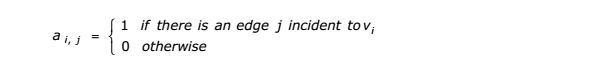
incidence matrix A is defined as an n by e matrix, say A = (ai,j), where
Here, n rows correspond to n vertices and e columns correspond to e edges. Such a
matrix is called as vertex-edge incidence matrix or simply incidence matrix.
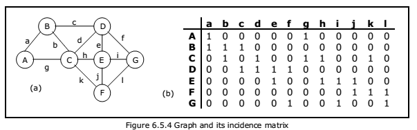
Figure 6.5.4(b) shows the incidence matrix representation of the graph G1 shown in
figure 6.5.4(a).